thar#
Here we will look at how to trace the RV drift of the spectrograph and correct for it.
This is very similar to the steps in the tempmatch example, but it is simpler as we do not have a target hurtling through space.
Again there’s a step-by-step example and a more compact version of function calls.
Step-by-step#
Spline creation#
import FIESpipe as fp
import numpy as np
import matplotlib.pyplot as plt
import scipy.interpolate as sci
path = 'your_path/to/spectra_and_tharframes/'
## Again, we'll start by grouping the spectra into
## science and ThAr files
filenames, tharnames = fp.sortFIES(path)
tharnames.sort()
## This time we'll use the ThAr files to
## create a master template to monitor
## the drift of the spectrograph
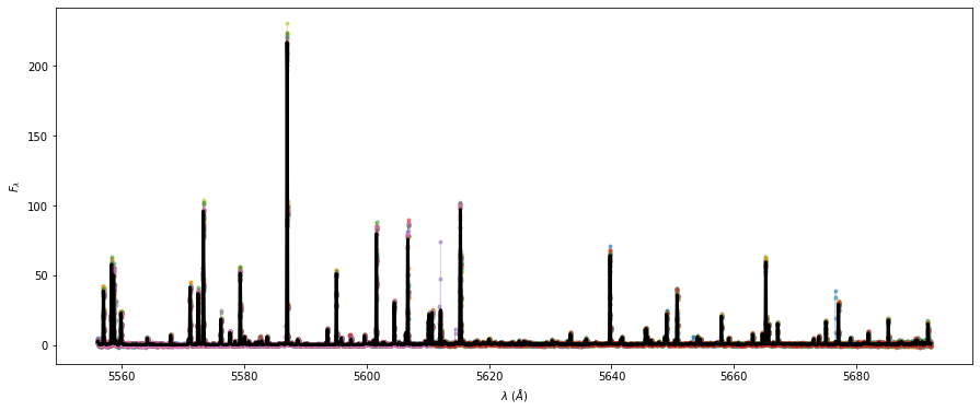
fig = plt.figure()
ax = fig.add_subplot(111)
ax.set_xlabel(r'$\lambda \ (\AA)$')
ax.set_ylabel(r'$F_\lambda$')
## We'll only plot orders in this interval
lo, ho = 51, 54
## As in some of the other examples
## this works best for the central orders
norders = range(40,60)
## Storage for splines
## and normalized ThAr spectra
splines = {}
prepped = {}
for file in tharnames:
prepped[file] = {}
for ii, order in enumerate(norders):
## Collect the wavelength and flux arrays
nwl = np.array([])
nfl = np.array([])
points = np.array([])
for jj, file in enumerate(tharnames):
## Extract the data from the FITS file
wave, flux, _, hdr = fp.extractFIES(file)
w = wave[order,:]
f = flux[order,:]
## Normalize the spectrum
nw, nf = fp.normalize(w,f)
prepped[file][order] = [nw,nf]
## Avoid cluttering the plot
if (order < ho) & (order > lo):
ax.plot(nw,nf,alpha=0.5,marker='.',lw=0.5)
nwl = np.append(nwl,nw)
nfl = np.append(nfl,nf)
points = np.append(points,len(w))
## How many points are in the wavelength
## Number of knots
Nknots = int(np.median(points))
## Sort the arrays by wavelength
ss = np.argsort(nwl)
nwl, nfl = nwl[ss], nfl[ss]
## Knots for the spline
knots = np.linspace(nwl[np.argmin(nwl)],nwl[np.argmax(nwl)],Nknots)
## Get the coefficients for the spline
t, c, k = sci.splrep(nwl, nfl, k=3, t=knots[4:-4])
## ...and create the spline
spline = sci.BSpline(t, c, k, extrapolate=False)
if (order < ho) & (order > lo):
ax.plot(nwl,spline(nwl),color='k',lw=3,zorder=5)
splines[order] = [nwl,spline]
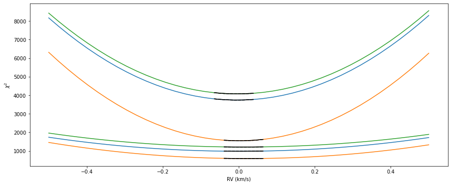
\(\chi^2\)-fitting#
## Dictionary to store the results
wrvs = {}
## Diagnostic plot
fig = plt.figure()
ax = fig.add_subplot(111)
ax.set_xlabel('RV (km/s)')
ax.set_ylabel(r'$\chi^2$')

## Points to include on either side of peak
pidx = 3

## Very narrow grid as the spectrograph
## (hopefully) doesn't drift too much
drvs = np.linspace(-0.5,0.5, 40)

## Loop over files
for ii, file in enumerate(tharnames):
        rvs = np.array([])
        ervs = np.array([])
        ## Loop over orders
        for jj, order in enumerate(norders):
                ## Collect the wavelength and spline
                twl, spline = splines[order]
                ## Normalized ThAr
                nwl, nfl = prepped[file][order]
                chi2s = np.array([])
                for drv in drvs:
                        ## Shift the spectrum
                        wl_shift = nwl/(1.0 + drv*1e3/fp.const.c.value)
                        mask = (wl_shift > min(twl)) & (wl_shift < max(twl))

                        ## Evaluate the spline at the shifted wavelength
                        ys = spline(wl_shift[mask])
                        ## There are no errors on the ThAr spectra
                        ## delivered by FIEStool
                        chi2 = np.sum((ys - nfl[mask])**2)
                        chi2s = np.append(chi2s,chi2)


                ## Find dip
                peak = np.argmin(chi2s)

                ## Don't use the entire grid, only points close to the minimum
                ## For bad CCFs, there might be several valleys
                ## in most cases the "real" RV should be close to the middle of the grid
                if (peak >= (len(chi2s) - pidx)) or (peak <= pidx):
                        peak = len(chi2s)//2
                keep = (drvs < drvs[peak+pidx]) & (drvs > drvs[peak-pidx])


                pars = np.polyfit(drvs[keep],chi2s[keep],2)
                if (order < ho) & (order > lo) & (ii < 3):
                        ax.plot(drvs,chi2s,color='C{}'.format(ii))
                        ax.plot(drvs[keep],chi2s[keep],color='k')
                        xx = np.linspace(min(drvs[keep]),max(drvs[keep]),100)
                        yy = np.polyval(pars,xx)
                        ax.plot(xx,yy,color='k',ls='--')

                ## The minimum of the parabola is the best RV
                rv = -pars[1]/(2*pars[0])
                ## The curvature is taking as the error.
                erv = np.sqrt(2/pars[0])
                if np.isfinite(rv) & np.isfinite(erv):
                        rvs = np.append(rvs,rv)
                        ervs = np.append(ervs,erv)
        wavg_rv, wavg_err, _, _  = fp.weightedMean(rvs,ervs,out=1,sigma=5)
        bjd, _ = fp.getBarycorrs(file,rvmeas=0.0)
        wrvs[file] = [bjd,wavg_rv,wavg_err]
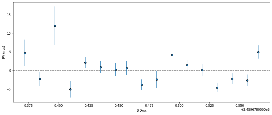
## This is how the RVs look
fig = plt.figure()
ax = fig.add_subplot(111)
ax.set_xlabel(r'$\mathrm{BJD}_\mathrm{TDB}$')
ax.set_ylabel(r'RV (m/s)')
ax.axhline(0.0,linestyle='--',color='C7')
## Collect RVs and timestamps
## to correct for the drift below
thimes = np.array([])
tharvs = np.array([])

for ii, file in enumerate(tharnames):
        bjd, rv, erv = wrvs[file]
        ax.errorbar(bjd,rv*1e3,yerr=erv*1e3,fmt='o',mfc='C0',mec='k',ecolor='C0')
        thimes = np.append(thimes,bjd)
        tharvs = np.append(tharvs,rv)

Applying the correction#
## In the following we'll use the RVs from the ThAr exposures
## to correct the drift in the RVs of the science exposures
## Here we'll assume that all science exposures are sandwiched between
## two ThAr exposures, which is also when it only really makes sense
dvs = np.array([])
for ii, file in enumerate(filenames):
        bjd, _ = fp.getBarycorrs(file,rvmeas=0.0)

        ## Find the two closest ThAr exposures
        close = np.argsort(np.abs(thimes - bjd))
        if bjd < thimes[close[0]]:
                after = close[0]
                before = close[1]
        else:
                after = close[1]
                before = close[0]

        ## Fractional distance between the two closest ThAr exposures
        frac = (bjd - thimes[before]) / (thimes[after] - thimes[before])
        ## The RV difference between the two closest ThAr exposures
        dv = (tharvs[after] - tharvs[before])*frac
        dvs = np.append(dvs,dv)

## These are then the corrections to be applied to the science RVs
Function calls#
import FIESpipe as fp
import numpy as np
import matplotlib.pyplot as plt
import scipy.interpolate as sci

## Set the path to the data and template
path = 'your_path/to/spectra/'

## Again, we'll start by grouping the spectra into
## science and ThAr files
filenames, tharnames = fp.sortFIES(path)
tharnames.sort()

## Again we'll start use some of the central orders
## (~5000-6000 AA)
norders = range(40,60)
## Prepare the ThAr spectra
prepped = fp.prepareThAr(tharnames,norders=norders)
## Create the splines
splines = fp.tharSplines(prepped,norders=norders)
## Get the RVs
wrvs = fp.thaRVs(prepped,splines)

## This is how the RVs look
fig = plt.figure(figsize=(width,height))
ax = fig.add_subplot(111)
ax.set_xlabel(r'$\mathrm{BJD}_\mathrm{TDB}$')
ax.set_ylabel(r'RV (m/s)')
ax.axhline(0.0,linestyle='--',color='C7')
## Collect RVs and timestamps
## to correct for the drift below
thimes = np.array([])
tharvs = np.array([])

for ii, file in enumerate(tharnames):
        bjd, rv, erv = wrvs[file]
        ax.errorbar(bjd,rv*1e3,yerr=erv*1e3,fmt='o',mfc='C0',mec='k',ecolor='C0')
        thimes = np.append(thimes,bjd)
        tharvs = np.append(tharvs,rv)
## In the following we'll use the RVs from the ThAr exposures
## to correct the drift in the RVs of the science exposures
## Here we'll assume that all science exposures are sandwiched between
## two ThAr exposures, which is also when it only really makes sense
dvs = np.array([])
bjds = np.array([])
for ii, file in enumerate(filenames):
        bjd, _ = fp.getBarycorrs(file,rvmeas=0.0)
        bjds = np.append(bjds,bjd)

dvs = fp.ThArcorr(thimes,tharvs,bjds)

## These are then the correction to the science RVs
- thar.thar(fpath='data/spectra/KELT-3/', save=False, width=15, height=6)#
Example showing how to correct for the ThAr Drift.
Used for testing.
- Parameters:
fpath (str) – Path to the FIES data. Default is
data/spectra/KELT-3/.save (bool) – Save the figures. Default is
False.width (float) – Width of the figures. Default is
15(inches).height (float) – Height of the figures. Default is
6(inches).
- Returns:
Correction to RVs.
- Return type:
array