broad#
An example of dealing with hotter stars with broader lines.
Example of how to use FIESpipe package on a faster rotating star – HAT-P-49.
The approach is the same as in basic to begin with, but eventually we use the broadening function to extract the line profile.
Normalization and outlier rejection#
>>> import FIESpipe as fp
>>> import matplotlib.pyplot as plt
>>> ## Sort the FIES files into science and ThAr spectra
>>> spec = 'your_path/HAT-P-49/'
>>> filenames, tharnames = fp.sortFIES(spec)
>>> filenames.sort()
>>> ## Run the standard reduction on the science spectra
>>> file = filenames[0]
>>> ## Extract the data from the FITS file
>>> wave, flux, ferr, hdr = fp.extractFIES(file)
>>> order = 45 #+1 # 0-indexed
>>> w, f, e = wave[order], flux[order], ferr[order]
>>> ## Relative error
>>> re = e/f
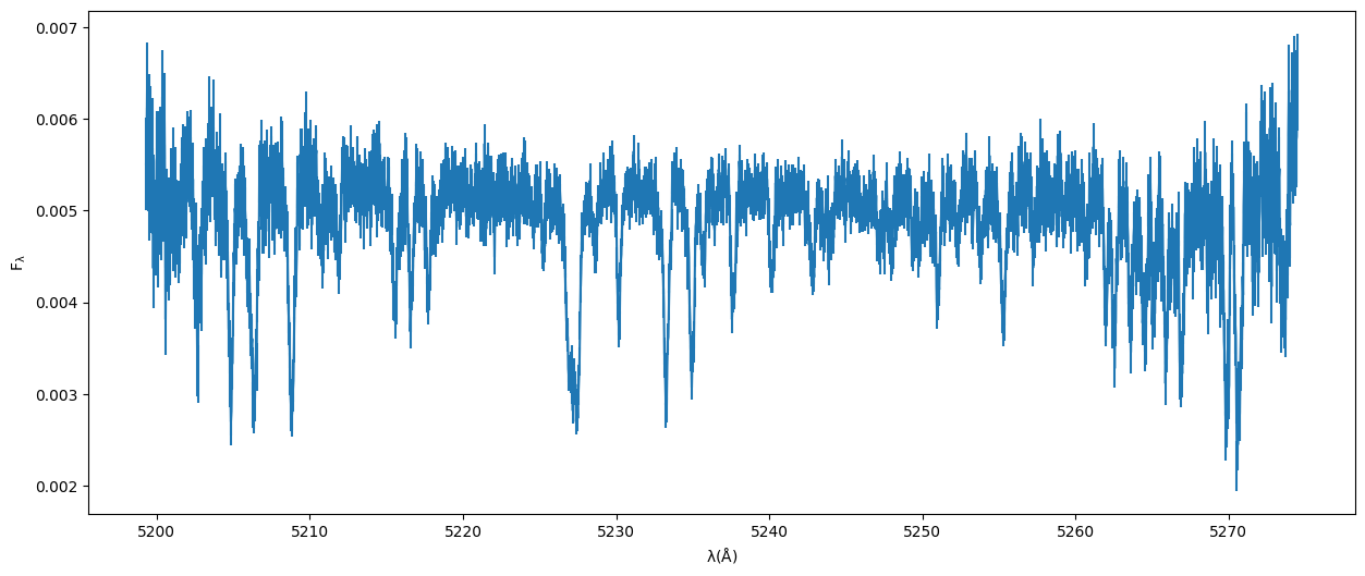
>>> ## Plot the spectrum
>>> fig = plt.figure()
>>> ax = fig.add_subplot(111)
>>> ax.set_xlabel(r'$\rm \lambda (\AA)$')
>>> ax.set_ylabel(r'$\rm F_{\lambda}$')
>>> ax.errorbar(w,f,yerr=e)
>>> ## Normalize the spectrum
>>> pdeg = 2 # Polynomial degree
>>> wl, nfl = fp.normalize(w,f,poly=pdeg)
>>> ## Scaled error
>>> nfle = re*nfl
>>> ## Cosmic ray removal/outlier rejection
>>> wlo, flo, eflo, idxs = fp.crm(wl,nfl,nfle)
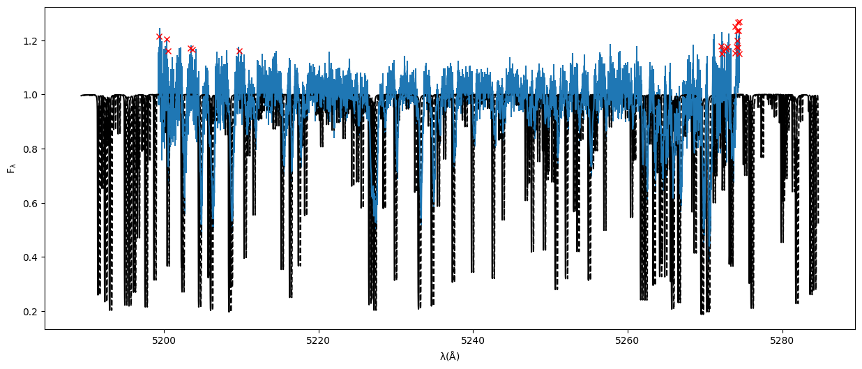
>>> ## Plot the normalized, cleansed spectrum
>>> fig = plt.figure()
>>> ax = fig.add_subplot(111)
>>> ax.set_xlabel(r'$\rm \lambda (\AA)$')
>>> ax.set_ylabel(r'$\rm F_{\lambda}$')
>>> ax.plot(wl[idxs],nfl[idxs],'rx',zorder=5)
>>> ## Plot the cleansed spectrum
>>> ax.errorbar(wlo,flo,yerr=eflo)
>>> ## Load Kurucz template
>>> temp = 'your_path/4750_30_p02p00.ms.fits'
>>> tw, tf = fp.readKurucz(temp)
>>> ## Plot the template in an interval around the order
>>> show = (tw > wlo.min()-5) & (tw < wlo.max()+5)
>>> ax.plot(tw[show],tf[show],'k-')
>>> ## For this star, I know the systemic velocity is around 15 km/s
>>> rvsys = 15 # km/s
>>> ## Shift the template to the systemic velocity,
>>> ### to center the grid around 0 km/s
>>> ### not important, but easier to work with
>>> sw = tw*(1.0 + rvsys*1e3/fp.const.c.value)
>>> ## Plot the shifted template
>>> ax.plot(sw[show],tf[show],'k--')
Cross-correlation function#
>>> ## Resample the template and the wavelength grid of the spectrum
>>> dv = fp.velRes(R=67000,s=2.1) # km/s, velocity resolution of the FIES spectrograph using fibre 4
>>> _, _, arvr, _, _, _ = fp.grids(rvr=201,R=67000,s=2.1) # velocity grid, range from 101 km/s
>>> lam, resamp_fl, resamp_tfl, resamp_fle = fp.resample(wl,nfl,nfle,sw,tf,dv=dv)
>>> rvs, ccf, errs = fp.getCCF(resamp_fl,resamp_tfl,resamp_fle,rvr=arvr,dv=dv)
>>> ## Plot the CCF
>>> fig = plt.figure()
>>> ax = fig.add_subplot(111)
>>> ax.set_xlabel(r'$\rm RV (km\,s^{-1})$')
>>> ax.set_ylabel(r'$\rm CCF$')
>>> ax.errorbar(rvs,ccf,yerr=errs)
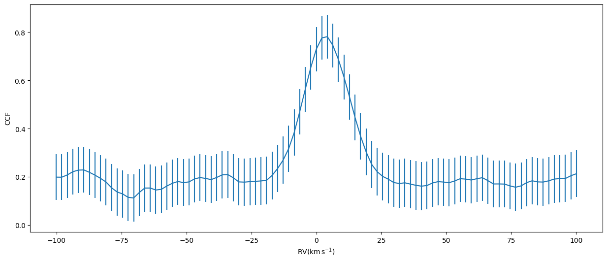
This was using the CCF, but let’s try the broadening function.
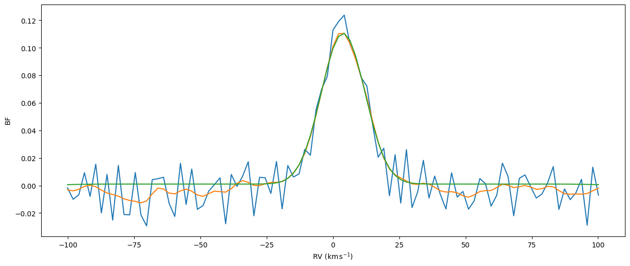
Broadening function#
>>> vel, bf = fp.getBF(resamp_fl,resamp_tfl,rvr=201,dv=dv)
>>> ## Plot the broadening function
>>> fig = plt.figure()
>>> ax = fig.add_subplot(111)
>>> ax.set_xlabel(r'$\rm RV \ (km\,s^{-1})$')
>>> ax.set_ylabel(r'$\rm BF$')
>>> ax.plot(vel,bf)
>>> ## Smooth the broadening function
>>> sm = 3#smoothing factor
>>> bfs = fp.smoothBF(vel,bf,sigma=sm)
>>> ## Plot the smoothed broadening function
>>> ax.plot(vel,bfs)
>>> ## Fit a rotation profile to the broadening function
>>> ## fit in an interval around the systemic velocity of +/-20 km/s
>>> ## Note the broadening function is smoothed by sm in this step
>>> fit, model, bfs = fp.rotBFfit(vel,bf,fitsize=20,smooth=sm,vsini=15)
>>> ## Plot the fit
>>> ax.plot(vel,model)
>>> ## Get the parameters of the fit
>>> amp = fit.params['ampl1'].value
>>> eamp = fit.params['ampl1'].stderr
>>> rv = fit.params['vrad1'].value
>>> erv = fit.params['vrad1'].stderr
>>> vsini = fit.params['vsini1'].value
>>> evsini = fit.params['vsini1'].stderr
>>> rv += rvsys
>>> ## Get the barycentric correction and BJD in TDB
>>> bjd, bvc = fp.getBarycorrs(file,rvmeas=rv)
>>> rv += bvc
>>> print('RV measured: {0:.3f} +/- {1:.3f} km/s'.format(rv,erv))
- broad.broad(fpath='data/spectra/HAT-P-49/', tpath='/6750_40_p00p00.ms.fits', save=False, width=15, height=6)#
Example using the broadening function.
Used for testing.
- Parameters:
fpath (str) – path to the FIES files
tpath (str) – path to the Kurucz template
save (bool) – save the plots
width (float) – Width of the figures. Default is
15(inches).height (float) – Height of the figures. Default is
6(inches).
- Returns:
RV, RV error, BJD, Barycentric correction, Amplitude, Amplitude error, vsini, vsini error
- Return type:
float, float, float, float, float, float, float, float