chisq#
An example showing how to extract RVs through \(\chi ^2\) minimization as used in, e.g., Zechmeister et al. (2018).
This example starts out similar to the one in basic, but then finds the RV through \(\chi ^2\) minimization.
Normalization and outlier rejection#
>>> import FIESpipe as fp
>>> import matplotlib.pyplot as plt
>>> import numpy as np
>>> ## Sort the FIES files into science and ThAr spectra
>>> spec = 'your_path/gamCep/'
>>> filenames, tharnames = fp.sortFIES(spec)
>>> filenames.sort()
>>> ## Run the standard reduction on the science spectra
>>> file = filenames[0]
>>> ## Extract the data from the FITS file
>>> wave, flux, ferr, hdr = fp.extractFIES(file)
>>> order = 45 #+1 # 0-indexed
>>> w, f, e = wave[order], flux[order], ferr[order]
>>> ## Relative error
>>> re = e/f
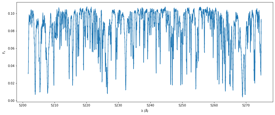
>>> ## Plot the spectrum
>>> fig = plt.figure()
>>> ax = fig.add_subplot(111)
>>> ax.set_xlabel(r'$\rm \lambda \ (\AA)$')
>>> ax.set_ylabel(r'$\rm F_{\lambda}$')
>>> ax.errorbar(w,f,yerr=e)
>>> ## Normalize the spectrum
>>> pdeg = 2 # Polynomial degree
>>> wl, nfl = fp.normalize(w,f,poly=pdeg)
>>> ## Scaled error
>>> nfle = re*nfl
>>> ## Cosmic ray removal/outlier rejection
>>> wlo, flo, eflo, idxs = fp.crm(wl,nfl,nfle)
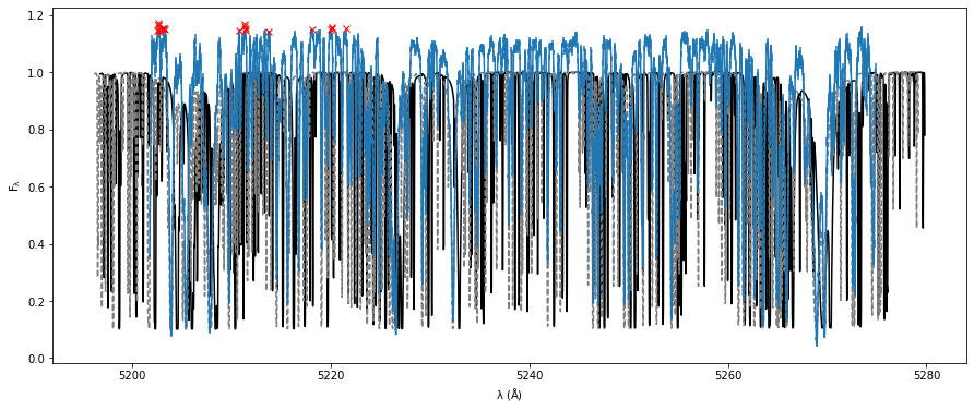
>>> ## Plot the normalized, cleansed spectrum
>>> fig = plt.figure()
>>> ax = fig.add_subplot(111)
>>> ax.set_xlabel(r'$\rm \lambda \ (\AA)$')
>>> ax.set_ylabel(r'$\rm F_{\lambda}$')
>>> ax.plot(wl[idxs],nfl[idxs],'rx',zorder=5)
>>> ## Plot the cleaned spectrum
>>> ax.errorbar(wlo,flo,yerr=eflo)
>>> ## Load Kurucz template
>>> temp = 'your_path/4750_30_p02p00.ms.fits'
>>> tw, tf = fp.readKurucz(temp)
>>> ## Plot the template in an interval around the order
>>> show = (tw > wlo.min()-5) & (tw < wlo.max()+5)
>>> ax.plot(tw[show],tf[show],'k-')
>>> ## For this star, I know the systemic velocity is around -40 km/s (+ the BVC...)
>>> rvsys = -36 # km/s
>>> ## Shift the template to the systemic velocity,
>>> ### to center the grid around 0 km/s
>>> ### not important, but easier to work with
>>> sw = tw*(1.0 + rvsys*1e3/fp.const.c.value)
>>> ## Plot the shifted template
>>> ax.plot(sw[show],tf[show],'--',color='C7')
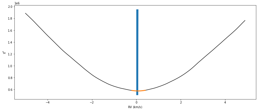
\(\chi ^2\) minimization#
>>> ## Find the best RV
>>> ## Through chi2 minimization
>>> ##Velocity grid to search
>>> drvs = np.arange(-5,5,0.1)
>>> ## Chi2 minimization for RVs
>>> chi2s = fp.chi2RV(drvs,wlo,flo,eflo,sw,tf)
>>> ## Plot the chi2 solutions
>>> fig = plt.figure()
>>> ax = fig.add_subplot(111)
>>> ax.set_xlabel(r'$\rm RV \ (km/s)$')
>>> ax.set_ylabel(r'$\rm \chi^2$')
>>> ax.plot(drvs,chi2s,'k-')
>>> ## Find dip
>>> peak = np.argmin(chi2s)
>>> ## Don't use the entire grid, only points close to the minimum
>>> ## For bad orders, there might be several valleys
>>> ## in most cases the "real" RV should be close to the middle of the grid
>>> pidx = 4 # Points to keep on each side of the minimum
>>> keep = (drvs < drvs[peak+pidx]) & (drvs > drvs[peak-pidx])
>>> ## Plot the minimum and the points to keep
>>> ax.plot(drvs[keep],chi2s[keep],color='C1',lw=3,zorder=5)
>>> ## Fit a parabola to the points to keep
>>> pars = np.polyfit(drvs[keep],chi2s[keep],2)
>>> ## The minimum of the parabola is the best RV
>>> rv = -pars[1]/(2*pars[0])
>>> ## The derivative/curvature is taking as the error.
>>> erv = np.sqrt(2/pars[0])
>>> ax.fill_betweenx(ax.get_ylim(),[rv-erv,rv+erv],color='C0')
>>> ## Remove the systemic velocity introduced earlier
>>> rv += rvsys
>>> ## Get the barycentric correction and BJD in TDB
>>> bjd, bvc = fp.getBarycorrs(file,rvmeas=rv)
>>> rv += bvc
>>> print('RV measured: {0:.3f} +/- {1:.3f} km/s'.format(rv,erv))
- chisq.chisq(fpath='data/spectra/gamCep/', tpath='/4750_30_p02p00.ms.fits', save=False, width=15, height=6)#
Example of RV extraction through \(\chi^2\) minimization.
Used for testing.
- Parameters:
fpath (str) – Path to the FIES data. Default is
data/spectra/gamCep/.tpath (str) – Path to the Kurucz template. Default is
/4750_30_p02p00.ms.fits.save (bool) – Save the figures. Default is
False.width (float) – Width of the figures. Default is
15(inches).height (float) – Height of the figures. Default is
6(inches).
- Returns:
RV, RV error, BJD, BVC, FWHM, FWHM error, contrast, contrast error
- Return type:
float, float, float, float, float, float, float, float