templates

In some of the other examples it was assumed that a template for the model atmosphere was available somewhere on the machine locally. However, we can also just download one given values for \(T_\mathrm{eff}\), \(\log g\), and \(\rm [Fe/H]\) (…and \([\alpha/\mathrm{Fe}]\)).

## Load the FIESpipe module
## and matplotlib for plotting
%matplotlib inline
import FIESpipe as fp
import matplotlib.pyplot as plt

Again we’ll be using the ATLAS9/Kurucz available here.

## Here we get the Kurucz model
## for a star with Teff=5500 K, logg=3.5, [Fe/H]=-1.1231, [alpha/Fe]=0.0
file = fp.getKurucz(5500, logg=3.5, feh=-1.1231, alpha=0.0)
## And as in the previous examples, we read the file
twl, tfl = fp.readKurucz(file)

## Let's plot the spectrum
fig = plt.figure(figsize=(14,6))
ax = fig.add_subplot(111)
ax.plot(twl, tfl)
ax.set_xlabel(r'$\lambda \ (\AA)$')
ax.set_ylabel(r'$F_\lambda$')

Text(0, 0.5, '$F_\\lambda$')

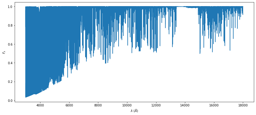
We can also use a PHOENIX template instead avaliable here. The wavelength for the PHOENIX template comes in a separate file, which will be downloaded in the same instance below.

## Here we get the Phoenix model
## for a star with Teff=5757 K, logg=3.8, [Fe/H]=-0.5, [alpha/Fe]=0.2
specfile, wavefile = fp.getPhoenix(5757,logg=3.8,feh=-0.5,alpha=0.2)
## Now we read the files
## We'll only read the wavelength range 5600-6800 Å
twl, tfl = fp.readPhoenix(specfile,wavefile,wl_min=5600,wl_max=6400)

## And plot the spectrum
fig = plt.figure(figsize=(14,6))
ax = fig.add_subplot(111)
ax.plot(twl, tfl)
ax.set_xlabel(r'$\lambda \ (\AA)$')
ax.set_ylabel(r'$F_\lambda$')

Text(0, 0.5, '$F_\\lambda$')

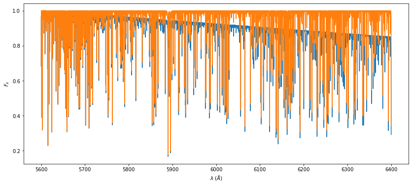
Evidently, this spectrum isn’t normalized. We can do this through continuum normalization using a max filter. This works best by grabbing chunks (as above) of the spectrum and not over the full wavelength range of the spectrum.

nfl = fp.contNormalize(twl, tfl, bins=100, pdeg=5)
## plot the normalized spectrum
fig = plt.figure(figsize=(14,6))
ax = fig.add_subplot(111)
ax.plot(twl, tfl)
ax.set_xlabel(r'$\lambda \ (\AA)$')
ax.set_ylabel(r'$F_\lambda$')
ax.plot(twl, nfl)

[<matplotlib.lines.Line2D at 0x7f2bfcf12fa0>]

Any other template (\(\lambda,F_\lambda\)) can, of course, also be used.