tempmatch

This is an example of how to extract RVs through template matching.

The idea is to construct a master template from the observations themselves. This is done through the creation of a spline which then constitutes an average high S/N spectrum of the target. This works best if the spline is created from many spectra at different epochs to account for changes in the lines.

This is similar to the approach in the SERVAL code (Zechmeister et al., 2018).

In the following examples we’ll look at observations of the planet host TOI-2158 discovered and characterized in Knudstrup et al. (2022). The spectra were acquired in sequences of three consecutive exposures of 15 min to better mitigate cosmic rays. An epoch is thus composed of three consecutive spectra. Therefore, we will also see how to \(\mathit{coadd}\) three spectra to create a single high S/N spectrum for a given epoch.

The following shows two examples on how to do this:

• the first is a step-by-step example outlining most of the steps in great detail,

• whereas the second example is a collection of calls to functions doing the same thing as in the first example

Note

The code takes a bit of time to compile – parallelize

Step-by-step

Normalization and initial RVs

import FIESpipe as fp
import numpy as np
import matplotlib.pyplot as plt
import scipy.interpolate as sci
import scipy.signal as scsig
import scipy.stats as scs
import os
path = os.path.dirname(os.path.abspath(__file__))

## Whether to save files
save = 0
## Figure format
width = 15
height = 6

## Here we'll group the data into epochs
## where an epoch in this case is a
## set of three spectra taken within
## an hour taken on a given night
fpath = 'data/spectra/TOI-2158/'
epochs = fp.groupByEpochs(path+'/../../'+fpath)

## We'll also create a list of the filenames
## for the initial preparation
filenames = []
for epoch in epochs:
        for file in epochs[epoch]['names']:
                filenames.append(file)

## Read in the template spectrum
temp = '4750_30_p02p00.ms.fits'
tw, tf = fp.readKurucz(path + '/../../data/temp/kurucz/' + temp)

## The orders used can influence the final RV
## and the error quite a bit
## We'll start out by using some of the
## (typically) well-behaved orders (~5000-6000 AA)
norders = range(40,60)

## We'll create a large and coarse grid
## to find the minimum of the chi2 function
## in RV
drvs_coarse = np.arange(-200,200,1)
pidx = 4 # Points to keep on each side of the minimum


## We'll create some diagnostic plots
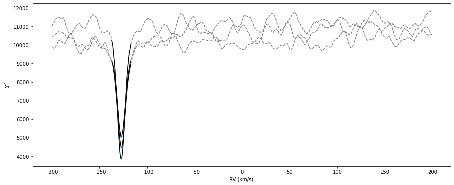
figchi = plt.figure(figsize=(width,height))
axchi = figchi.add_subplot(111)
axchi.set_xlabel('RV (km/s)')
axchi.set_ylabel(r'$\chi^2$')

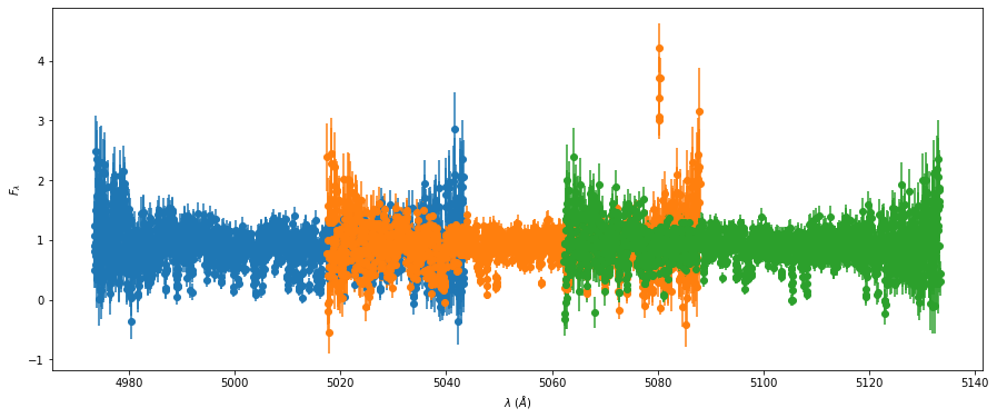
figsp = plt.figure(figsize=(width,height))
axsp = figsp.add_subplot(111)
axsp.set_xlabel(r'$\lambda \ (\AA)$')
axsp.set_ylabel(r'$F_{\lambda}$')


## Dictionary to store the prepped data
## normalized spectra/initial RVs
prepped = {
                'orders':norders,
                'files':filenames
}
for ii, file in enumerate(filenames):
        ## Extract the data from the FITS file
        wave, flux, ferr, hdr = fp.extractFIES(file)
        rvs = np.array([])
        ervs = np.array([])
        prepped[file] = {
                'bjd':np.nan,
                'rv':np.nan,
                'erv':np.nan,
        }
        for jj, order in enumerate(norders):
                w, f, e = wave[order], flux[order], ferr[order]
                ## Relative error
                re = e/f
                ## Normalize the spectrum
                wl, nfl = fp.normalize(w,f)
                ## Scaled error
                nfle = re*nfl

                ## Plot the normalized spectrum
                ## but avoid clutter
                if not ii:
                        if jj < 3:
                                axsp.errorbar(wl,nfl,yerr=nfle,fmt='o')

                ## Save the prepped spectrum
                prepped[file][order] = {
                        'wave': wl,
                        'flux': nfl,
                        'err': nfle,
                }
                ## Cosmic ray removal/outlier rejection
                ## Here only used to get the first guess for the RV
                wlo, flo, eflo, idxs = fp.crm(wl,nfl,nfle)

                ## Chi2 minimization for RVs
                chi2s_c = fp.chi2RV(drvs_coarse,wlo,flo,eflo,tw,tf)
                if not ii:
                        if jj < 3:
                                axchi.plot(drvs_coarse,chi2s_c,'--',color='C7')

                ## Find dip
                peak_c = np.argmin(chi2s_c)
                ## Finer grid
                drvs = np.arange(drvs_coarse[peak_c-10],drvs_coarse[peak_c+10],0.1)
                chi2s = fp.chi2RV(drvs,wlo,flo,eflo,tw,tf)
                if not ii:
                        if jj < 3:
                                axchi.plot(drvs,chi2s,'k-')
                peak = np.argmin(chi2s)

                ## Don't use the entire grid, only points close to the minimum
                ## For bad orders, there might be several valleys
                ## in most cases the "real" RV should be close to the middle of the grid
                keep = (drvs < drvs[peak+pidx]) & (drvs > drvs[peak-pidx])

                ## Plot the minimum and the points to keep
                if not ii:
                        if jj < 3:
                                axchi.plot(drvs[keep],chi2s[keep],color='C0',lw=3,zorder=5)

                ## Fit a parabola to the points to keep
                pars = np.polyfit(drvs[keep],chi2s[keep],2)

                ## The minimum of the parabola is the best RV
                rv = -pars[1]/(2*pars[0])
                ## The curvature is taking as the error.
                erv = np.sqrt(2/pars[0])
                if np.isfinite(rv) & np.isfinite(erv):
                        rvs = np.append(rvs,rv)
                        ervs = np.append(ervs,erv)

        wavg_rv, wavg_err, _, _  = fp.weightedMean(rvs,ervs,out=1,sigma=5)

        ## Get BJD_TDB
        bjd, _ = fp.getBarycorrs(file,wavg_rv)
        prepped[file]['bjd'] = bjd
        prepped[file]['rv'] = wavg_rv
        prepped[file]['erv'] = wavg_err


if save:
        figchi.savefig('./chi2_ini.png',bbox_inches='tight')
        figsp.savefig('./spec_ini.png',bbox_inches='tight')

Spline creation - 1st iteration

#%%
## Now we'll use all these prepped spectra
## to create the first iteration of splines
splines = {}
## Again some diagnostic plots
figspl = plt.figure(figsize=(width,height))
axspl = figspl.add_subplot(111)
axspl.set_xlabel(r'$\lambda \ (\AA)$')
axspl.set_ylabel(r'$F_{\lambda}$')

## Loop over orders
for ii, order in enumerate(norders):
        ## Collect wavelength, flux, and error arrays
        swl = np.array([])
        fl = np.array([])
        fle = np.array([])
        ## and the number of points in each spectrum
        points = np.array([])
        ## Loop over files
        for jj, file in enumerate(filenames):
                wl, nfl, nfle = prepped[file][order]['wave'], prepped[file][order]['flux'], prepped[file][order]['err']
                ## Get derived RV
                rv = prepped[file]['rv']
                ## Shift the spectrum according to the measured velocity
                nwl = wl*(1.0 - rv*1e3/fp.const.c.value)

                swl = np.append(swl,nwl)
                fl = np.append(fl,nfl)
                fle = np.append(fle,nfle)
                points = np.append(points,len(wl))

        ## How many points are in the wavelength
        points = np.median(points)

        ## Sort the arrays by wavelength
        ss = np.argsort(swl)
        swl, fl, fle = swl[ss], fl[ss], fle[ss]

        ## Again avoid clutter
        if ii < 3:
                axspl.errorbar(swl,fl,yerr=fle,fmt='o')

        ## Weights
        w = 1.0/fle

        ## Number of knots,
        ## just use the median number of points in wavelength
        Nknots = int(points)

        ## The following is a bit hacky
        ## The idea is to try to get as close to the knots as returned by the SERVAL spline
        ## The knots have to be within the range of the wavelength array
        ## ... this "hackiness" includes the knots[4:-4]
        knots = np.linspace(swl[np.argmin(swl)],swl[np.argmax(swl)],Nknots)

        ## Get the coefficients for the spline
        t, c, k = sci.splrep(swl, fl, w=w, k=3, t=knots[4:-4])
        ## ...and create the spline
        spline = sci.BSpline(t, c, k, extrapolate=False)
        if ii < 3:
                axspl.plot(swl,spline(swl),color='k',lw=2,zorder=5)

        splines[order] = [swl,spline]

if save:
        figspl.savefig('./splines_ini.png',bbox_inches='tight')

RVs from splines - 1st iteration

## Now we'll use the splines as a template
## to get the RVs
## The procedure is very similar to the one above

## Dictionary to store the results
wrvs = {}
## Diagnostic plot
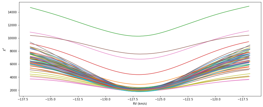
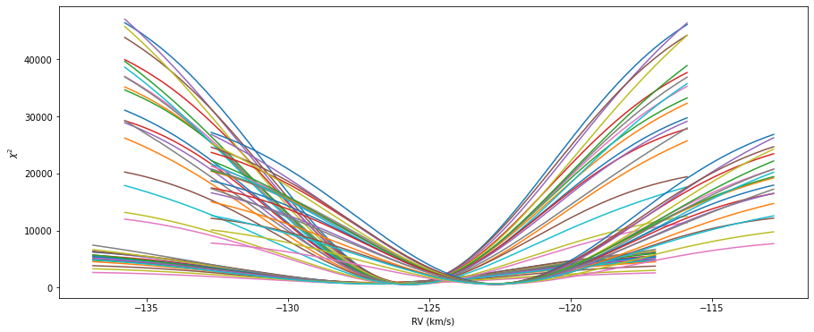
figchi = plt.figure(figsize=(width,height))
axchi = figchi.add_subplot(111)
axchi.set_xlabel('RV (km/s)')
axchi.set_ylabel(r'$\chi^2$')
## Loop over files
for ii, file in enumerate(filenames):
        ## Get derived RV
        wrv = prepped[file]['rv']
        ## We'll use a finer grid
        ## around the measured RV
        drvs = np.arange(wrv-10,wrv+10,0.1)

        ## Loop over orders
        rvs = np.array([])
        ervs = np.array([])
        for jj, order in enumerate(norders):
                ## Collect the wavelength and spline
                twl, spline = splines[order]
                ## Extract the wavelength, flux, and error arrays
                wl, nfl, nfle = prepped[file][order]['wave'], prepped[file][order]['flux'], prepped[file][order]['err']

                chi2s = np.array([])
                for drv in drvs:
                        ## Shift the spectrum
                        wl_shift = wl/(1.0 + drv*1e3/fp.const.c.value)
                        mask = (wl_shift > min(twl)) & (wl_shift < max(twl))
                        ## Evaluate the spline at the shifted wavelength
                        ys = spline(wl_shift[mask])
                        chi2 = np.sum((ys - nfl[mask])**2/nfle[mask]**2)
                        chi2s = np.append(chi2s,chi2)

                if ii < 3:
                        axchi.plot(drvs,chi2s)

                ## Find dip
                peak = np.argmin(chi2s)

                ## Don't use the entire grid, only points close to the minimum
                ## For bad CCFs, there might be several valleys
                ## in most cases the "real" RV should be close to the middle of the grid
                if (peak >= (len(chi2s) - pidx)) or (peak <= pidx):
                        peak = len(chi2s)//2
                keep = (drvs < drvs[peak+pidx]) & (drvs > drvs[peak-pidx])

                pars = np.polyfit(drvs[keep],chi2s[keep],2)

                ## The minimum of the parabola is the best RV
                rv = -pars[1]/(2*pars[0])
                ## The curvature is taking as the error.
                erv = np.sqrt(2/pars[0])
                if np.isfinite(rv) & np.isfinite(erv):
                        rvs = np.append(rvs,rv)
                        ervs = np.append(ervs,erv)
        wavg_rv, wavg_err, _, _  = fp.weightedMean(rvs,ervs,out=1,sigma=5)
        bjd, bvc = fp.getBarycorrs(file,wavg_rv)
        wrvs[file] = [bjd,wavg_rv,wavg_err,bvc]

if save:
        figchi.savefig('./chi2_second.png',bbox_inches='tight')

Spline creation - 2nd iteration

## We'll now use the newly derived RVs
## in the second iteration
for file in wrvs:
        bjd, rv, erv, bvc = wrvs[file]
        prepped[file]['rv'] = rv
        prepped[file]['erv'] = erv
## and we'll make a new batch of splines

## Diagnostic plot
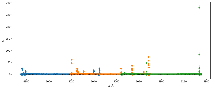
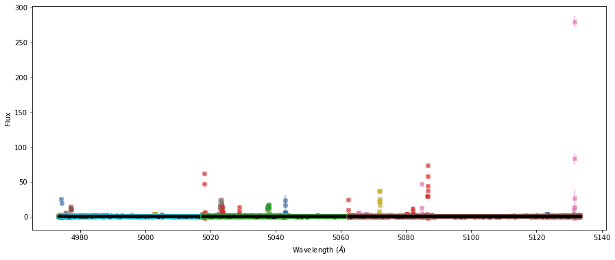
figspl = plt.figure(figsize=(width,height))
axspl = figspl.add_subplot(111)
axspl.set_xlabel(r'Wavelength ($\AA$)')
axspl.set_ylabel('Flux')

## New dictionary to store the splines
second = {}
## The procedure is exactly the same as to the one above
## but this time there will be on iteration of outlier rejection
## Loop over orders
for ii, order in enumerate(norders):
        ## Collect wavelength, flux, and error arrays
        swl = np.array([])
        fl = np.array([])
        fle = np.array([])
        ## and the number of points in each spectrum
        points = np.array([])
        ## Loop over files
        for jj, file in enumerate(filenames):
                wl, nfl, nfle = prepped[file][order]['wave'], prepped[file][order]['flux'], prepped[file][order]['err']
                ## Get derived RV
                rv = prepped[file]['rv']
                ## Shift the spectrum according to the measured velocity
                nwl = wl*(1.0 - rv*1e3/fp.const.c.value)
                if ii < 3:
                        axspl.errorbar(nwl,nfl,nfle,color='C{}'.format(ii),alpha=0.3)

                swl = np.append(swl,nwl)
                fl = np.append(fl,nfl)
                fle = np.append(fle,nfle)
                points = np.append(points,len(wl))

        ## How many points are in the wavelength
        points = np.median(points)

        ## Sort the arrays by wavelength
        ss = np.argsort(swl)
        swl, fl, fle = swl[ss], fl[ss], fle[ss]

        for jj in range(1):
                ## Savitzky-Golay filter for outlier rejection
                yhat = scsig.savgol_filter(fl, 51, 3)
                res = fl-yhat

                ## Rejection
                mu, sig = scs.norm.fit(res)
                sig *= 5
                keep = (res < (mu + sig)) & (res > (mu - sig))

                if ii < 3:
                        axspl.errorbar(swl[~keep], fl[~keep], yerr=fle[~keep],fmt='x',color='C3')
                ## Trim the arrays
                swl, fl, fle = swl[keep], fl[keep], fle[keep]

        ## Weights
        w = 1.0/fle

        ## Number of knots,
        ## just use the median number of points in wavelength
        Nknots = int(points)

        ## The following is a bit hacky
        ## The idea is to try to get as close to the knots as returned by the SERVAL spline
        ## The knots have to be within the range of the wavelength array
        ## ... this "hackiness" includes the knots[4:-4]
        knots = np.linspace(swl[np.argmin(swl)],swl[np.argmax(swl)],Nknots)

        ## Get the coefficients for the spline
        t, c, k = sci.splrep(swl, fl, w=w, k=3, t=knots[4:-4])
        ## ...and create the spline
        spline = sci.BSpline(t, c, k, extrapolate=False)

        ## Plot the spline
        if ii < 3:
                axspl.plot(swl,spline(swl),color='k')
        second[order] = [swl,spline]

if save:
        figchi.savefig('./spline_second.png',bbox_inches='tight')

Coadd epochs

Note

The coadding here is done in a way that assumes that the spectra in the epoch have the exact same wavelength solution. A way to go about this would be to find the nearest neighbours for a given wavelength step. See highlighted comments below.

## We could now use the splines to get the RVs for each individual spectrum again,
## but this time we'll coadd the spectra from different epochs first

## Store the coadded spectra in a dictionary
coadd = {}
## Diagnostic plot
figco = plt.figure(figsize=(width,height))
axco = figco.add_subplot(111)
axco.set_xlabel(r'Wavelength ($\AA$)')
axco.set_ylabel('Flux')

## Loop over epochs
for epoch in epochs:
        filenames = epochs[epoch]['names']

        coadd[epoch] = {'files':filenames,'orders':norders}
        rv = np.array([])
        for file in filenames:
                rv = np.append(rv,prepped[file]['rv'])
        ## Get the median RV for the epoch
        coadd[epoch]['rv'] = np.median(rv)
        ## For each order append flux and errors for each file
        for ii, order in enumerate(prepped['orders']):
                wls = np.array([])
                fls = np.array([])
                fles = np.array([])
                for jj, file in enumerate(filenames):
                        wl = prepped[file][order]['wave']
                        fl = prepped[file][order]['flux']
                        fle = prepped[file][order]['err']
                        ## Append the arrays
                        wls = np.append(wls,wl)
                        fls = np.append(fls,fl)
                        fles = np.append(fles,fle)
                        if ii < 3:
                                axco.errorbar(wl,fl,yerr=fle,fmt='o',alpha=0.5)

                ## Copy the wavelength array
                ## To keep track of indices
                wlc = wl.copy()

                ## Outlier rejection
                for jj in range(2):
                        ## Savitzky-Golay filter for outlier rejection
                        yhat = scsig.savgol_filter(fls, 51, 3)
                        res = fls-yhat

                        ## Rejection
                        mu, sig = scs.norm.fit(res)
                        sig *= 5
                        keep = (res < (mu + sig)) & (res > (mu - sig))
                        if ii < 3:
                                axco.plot(wls[~keep], fls[~keep],marker='x',color='C3',ls='none',alpha=0.5)
                        ## Trim the arrays
                        wls, fls, fles = wls[keep], fls[keep], fles[keep]

                ## Coadd the spectra
                fwls = np.array([])
                ffls = np.array([])
                ferr = np.array([])
                ## Loop over the wavelengths
                ## if wavelength is still in the array
                ## take the mean of the fluxes
                ## and append to the arrays
                for jj, wl in enumerate(wlc):
                        idxs = np.where(wls == wl)[0]
                        ## Alternatively, it would be something along the line
                        ## idxs = np.where(np.abs(wls-wl)<deltaWL)[0]
                        ## where deltaWL is some threshold
                        ## Could be set to be a fraction of the median spacing
                        ## between wavelength points in each of the spectra

                        if len(idxs):
                                ## If the wavelength steps are not the same
                                ## then it should be
                                ## fwls = np.append(fwls,np.mean(wls[idxs]))
                                fwls = np.append(fwls,wl)
                                ffls = np.append(ffls,np.mean(fls[idxs]))
                                ## Propagate the errors
                                ferr = np.append(ferr,np.sqrt(np.sum(fles[idxs]**2)/len(idxs)))
                if ii < 3:
                        axco.errorbar(fwls,ffls,yerr=ferr,alpha=0.5,color='k',ls='--',marker='.')
                ## Append the coadded spectrum to the dict
                coadd[epoch][order] = {'wave':fwls,'flux':ffls,'err':ferr}
# %%
if save:
        figco.savefig('./coadd.png',bbox_inches='tight')

Final RV extraction

## Finally, we'll loop over the coadded spectra
## and get the RVs using our splines create from the individual spectra

## Diagnostic plot
figchi = plt.figure(figsize=(width,height))
axchi = figchi.add_subplot(111)
axchi.set_xlabel('RV (km/s)')
axchi.set_ylabel(r'$\chi^2$')

## We'll store the weighted average RV and error
## for each epoch in arrays
final_rvs = np.array([])
final_ervs = np.array([])
## As well as the time and barycentric correction
final_bjds = np.array([])
final_bvcs = np.array([])
## Loop over epochs
for ii, epoch in enumerate(epochs):
        filenames = epochs[epoch]['names']

        ## Fine grid around the measured RV
        rvepoch = coadd[epoch]['rv']
        drvs = np.arange(rvepoch - 10.0, rvepoch + 10.0, 0.1)
        ## Loop over orders
        rvs = np.array([])
        ervs = np.array([])
        for jj, order in enumerate(norders):
                ## Collect the wavelength and spline
                twl, spline = second[order]
                ## Extract the wavelength, flux, and error arrays
                wl, nfl, nfle = coadd[epoch][order]['wave'], coadd[epoch][order]['flux'], coadd[epoch][order]['err']

                chi2s = np.array([])
                for drv in drvs:
                        ## Shift the spectrum
                        wl_shift = wl/(1.0 + drv*1e3/fp.const.c.value)
                        mask = (wl_shift > min(twl)) & (wl_shift < max(twl))
                        ## Evaluate the spline at the shifted wavelength
                        ys = spline(wl_shift[mask])
                        chi2 = np.sum((ys - nfl[mask])**2/nfle[mask]**2)
                        chi2s = np.append(chi2s,chi2)

                if ii < 3:
                        axchi.plot(drvs,chi2s)
                ## Find dip
                peak = np.argmin(chi2s)

                ## Don't use the entire grid, only points close to the minimum
                ## For bad CCFs, there might be several valleys
                ## in most cases the "real" RV should be close to the middle of the grid
                if (peak >= (len(chi2s) - pidx)) or (peak <= pidx):
                        peak = len(chi2s)//2
                keep = (drvs < drvs[peak+pidx]) & (drvs > drvs[peak-pidx])

                pars = np.polyfit(drvs[keep],chi2s[keep],2)

                ## The minimum of the parabola is the best RV
                rv = -pars[1]/(2*pars[0])
                ## The curvature is taking as the error.
                erv = np.sqrt(2/pars[0])
                if np.isfinite(rv) & np.isfinite(erv):
                        rvs = np.append(rvs,rv)
                        ervs = np.append(ervs,erv)

        wavg_rv, wavg_err, _, _  = fp.weightedMean(rvs,ervs,out=1,sigma=5)

        ## We'll also extract the BJD in TDB
        ## and the barycentric correction
        ## Which here is the mean of the spectra comprising up the epoch
        bjds = np.array([])
        bvcs = np.array([])
        for file in filenames:
                bjd, bvc = fp.getBarycorrs(file,wavg_rv)
                bjds = np.append(bjds,bjd)
                bvcs = np.append(bvcs,bvc)

        final_bjds = np.append(final_bjds,np.mean(bjds))
        final_bvcs = np.append(final_bvcs,np.mean(bvcs))
        final_rvs = np.append(final_rvs,wavg_rv+np.mean(bvcs))
        final_ervs = np.append(final_ervs,wavg_err)

if save:
        figchi.savefig('./chi2_final.png',bbox_inches='tight')

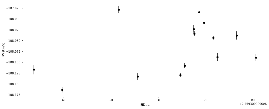
## Plot and the final RVs
print(final_rvs,final_ervs)

fig = plt.figure(figsize=(width,height))
ax = fig.add_subplot(111)
ax.set_xlabel(r'$\mathrm{BJD}_\mathrm{TDB}$')
ax.set_ylabel(r'RV (km/s)')
ax.errorbar(final_bjds,final_rvs,yerr=final_ervs,fmt='o',color='k')
if save:
        fig.savefig('./rvs.png',bbox_inches='tight')
        ## and save the RVs to a file
        arr = np.array([final_bjds,final_rvs,final_ervs]).T
        #np.savetxt('./rvs.txt',arr)

Function calls

>>> import FIESpipe as fp
>>> import numpy as np
>>> import matplotlib.pyplot as plt
>>> import glob

>>> ## Set the path to the data and template
>>> path = 'your_path/TOI-2158/'
>>> ## Group the spectra by epoch
>>> epochs = fp.groupByEpochs(path)
>>> ## We'll also create a list of the filenames
>>> ## for the initial preparation
>>> filenames = glob.glob(path+'*wave.fits')
>>> ## Load Kurucz template
>>> tpath = '/4750_30_p02p00.ms.fits'
>>> tw, tf = fp.readKurucz(path + 'kurucz/' + tpath)

>>> ## The orders used can influence the final RV
>>> ## and the error quite a bit
>>> ## We'll start out by using some of the
>>> ## (typically) well-behaved orders (~5000-6000 AA)
>>> norders = range(40,60)

>>> ## Dictionary to store the prepped data
>>> ## normalized spectra/initial RVs
>>> prepped = fp.prepareSpectra(filenames,norders,tw,tf)

>>> ## Now we'll use all these prepped spectra
>>> ## to create the first iteration of splines
>>> splines = fp.makeSplines(prepped)

>>> ## Now we'll use the splines as a template
>>> ## to get the RVs
>>> ## The procedure is very similar to the one above

>>> ## Dictionary to store the results
>>> wrvs = fp.matchRVs(prepped,splines)

>>> ## We'll now use the newly derived RVs
>>> ## in the second iteration
>>> for file in wrvs:
>>>     bjd, rv, erv, bvc = wrvs[file]
>>>     prepped[file]['rv'] = rv
>>>     prepped[file]['erv'] = erv
>>> ## and we'll make a new batch of splines

>>> ## New dictionary to store the splines
>>> second = fp.makeSplines(prepped)

>>> ## We could now use the splines to get the RVs for each individual spectrum again,
>>> ## but this time we'll coadd the spectra from different epochs first
>>> ## We'll store the weighted average RV and error
>>> ## for each epoch in arrays
>>> final_rvs = np.array([])
>>> final_ervs = np.array([])
>>> ## As well as the time and barycentric correction
>>> final_bjds = np.array([])
>>> final_bvcs = np.array([])
>>> for epoch in epochs:
>>>     filenames = epochs[epoch]['names']
>>>     ## Fine grid centered on the measrued RV
>>>     rv = np.array([])
>>>     for file in filenames:
>>>             rv = np.append(rv,prepped[file]['rv'])
>>>     rvepoch = np.median(rv)
>>>     drvs = np.arange(rvepoch - 10.0, rvepoch + 10.0, 0.1)
>>>     ## Coadd the spectra
>>>     coadd = fp.coaddSpectra(filenames,prepped)
>>>     ## Get the RVs
>>>     wavg_rv, wavg_err = fp.splineRVs(coadd,second,drvs)
>>>     ## Get the barycentric correction
>>>     ## and the BJD in TDB
>>>     bjds = np.array([])
>>>     bvcs = np.array([])
>>>     for file in filenames:
>>>             bjd, bvc = fp.getBarycorrs(file,wavg_rv)
>>>             bjds = np.append(bjds,bjd)
>>>             bvcs = np.append(bvcs,bvc)
>>>     ## ... this could be done in a more sophisticated way
>>>     ## by for example using the flux weighted midpoint of the exposure
>>>     ## but this is good enough for now
>>>     ## Append to arrays
>>>     final_bjds = np.append(final_bjds,np.mean(bjds))
>>>     final_bvcs = np.append(final_bvcs,np.mean(bvcs))
>>>     final_rvs = np.append(final_rvs,wavg_rv+np.mean(bvcs))
>>>     final_ervs = np.append(final_ervs,wavg_err)

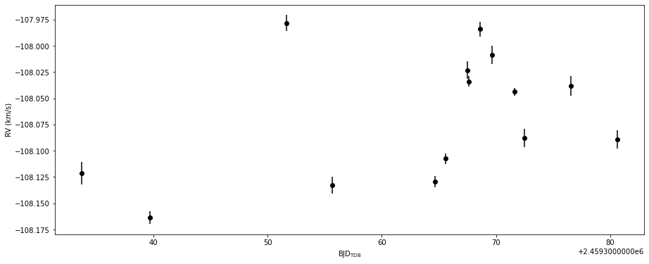
>>> for ii, bjd in enumerate(final_bjds):
>>>     print('BJD: {:.5f}, RV: {:.3f} +/- {:.3f} m/s'.format(bjd,final_rvs[ii]*1e3,final_ervs[ii]*1e3))

BJD: 2459333.70360, RV: -108121.328 +/- 10.511 m/s
BJD: 2459339.68180, RV: -108163.728 +/- 5.878 m/s
BJD: 2459351.64286, RV: -107978.377 +/- 7.666 m/s
BJD: 2459355.66056, RV: -108132.583 +/- 7.999 m/s
BJD: 2459364.63371, RV: -108129.309 +/- 5.484 m/s
BJD: 2459365.60471, RV: -108107.542 +/- 4.827 m/s
BJD: 2459367.51570, RV: -108023.135 +/- 8.147 m/s
BJD: 2459367.64103, RV: -108033.972 +/- 5.167 m/s
BJD: 2459368.63520, RV: -107984.135 +/- 6.939 m/s
BJD: 2459369.68646, RV: -108008.666 +/- 8.646 m/s
BJD: 2459371.62623, RV: -108043.780 +/- 3.844 m/s
BJD: 2459372.49619, RV: -108087.778 +/- 8.811 m/s
BJD: 2459376.59300, RV: -108037.943 +/- 9.436 m/s
BJD: 2459380.64168, RV: -108088.978 +/- 8.693 m/s

>>> ## Plot the RVs
>>> fig = plt.figure(figsize=(width,height))
>>> ax = fig.add_subplot(111)
>>> ax.errorbar(final_bjds,final_rvs,yerr=final_ervs,fmt='o',color='k')
>>> ax.set_xlabel(r'$\mathrm{BJD}_\mathrm{TDB}$')
>>> ax.set_ylabel(r'RV (km/s)')

tempmatch.tempmatch(fpath='data/spectra/TOI-2158/', tpath='/4750_30_p02p00.ms.fits', save=False, width=15, height=6)

Example of the FIESpipe package for template matching.

Used for testing.

Parameters:

• fpath (str) – Path to the FIES data. Default is data/spectra/TOI-2158/.

• tpath (str) – Path to the Kurucz template. Default is /4750_30_p02p00.ms.fits.

• save (bool) – Save the figures. Default is False.

• width (float) – Width of the figures. Default is 15 (inches).

• height (float) – Height of the figures. Default is 6 (inches).

Returns:

BJD, RVs, RV errors, BVC

Return type:

array, array, array, array